Basic example

Let us demonstrate the basic usage of hdnet using the following example. The source code for this example can be found in this example script in the examples/ directory.

For demonstration purposes we will start work with a synthetic data set in this tutorial (later we will be working with real spiking data). Spiking activity of 10 hypothetical cells is assumed to be given as independent, identically distributed (i.i.d.) Poisson processes. Upon binning with a given bin width, this yields Bernoulli processes in discrete time. We create such Bernoulli data (as a proxy for real, binned spiking data) and then insert hypothetical correlations by means of a number of co-activations of different cell groups over time (also known as cell assemblies).

Starting off

We first import the necessary modules into our Python session (we recommend using ipython in pylab mode, i.e. running ipython --pylab and to run text copied to the clipboard from this tutorial using the magic command %paste):

import numpy as np
import matplotlib.pyplot as plt
from hdnet.stimulus import Stimulus
from hdnet.spikes import Spikes
from hdnet.spikes_model import SpikeModel, BernoulliHomogeneous, DichotomizedGaussian

Next, we create two trials of 200 time bins of spikes from 10 neurons and store them in a Spikes container:

# Let's first make up some simuilated spikes: 2 trials
spikes = (np.random.random((2, 10, 200)) < .05).astype(int)
spikes[0, [1, 5], ::5] = 1  # insert correlations
spikes[1, [2, 3, 6], ::11] = 1  # insert correlations

spikes = Spikes(spikes=spikes)

We can now plot a raster of the trials and covariances:

# let's look at the raw spikes and their covariance
plt.figure()
plt.matshow(spikes.rasterize(), cmap='gray')
plt.title('Raw spikes')

plt.figure()
plt.matshow(spikes.covariance().reshape((2 * 10, 10)), cmap='gray')
plt.title('Raw spikes covariance')
plt.show()

Next, we would like to model this noisy binary data. First, we try to model each trial with a separate i.i.d. Bernoulli random binary vector having the same neuron means as in each trial:

# let's examine the structure in spikes using a spike modeler
spikes_model = BernoulliHomogeneous(spikes=spikes)
BH_sample_spikes = spikes_model.sample_from_model()

plt.figure()
plt.matshow(BH_sample_spikes.rasterize(), cmap='gray')
plt.title('BernoulliHomogeneous sample')
print "%1.4f means" % BH_sample_spikes.spikes.mean()

plt.figure()
plt.matshow(BH_sample_spikes.covariance().reshape((2 * 10, 10)), cmap='gray')
plt.title('BernoulliHomogeneous covariance')

plt.show()

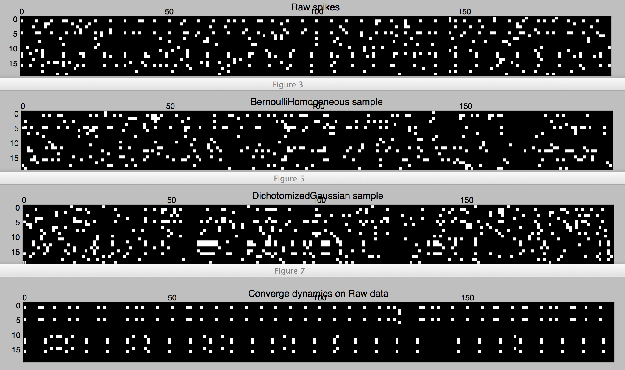
Figure 1. Spikes of two trials with 10 neurons.

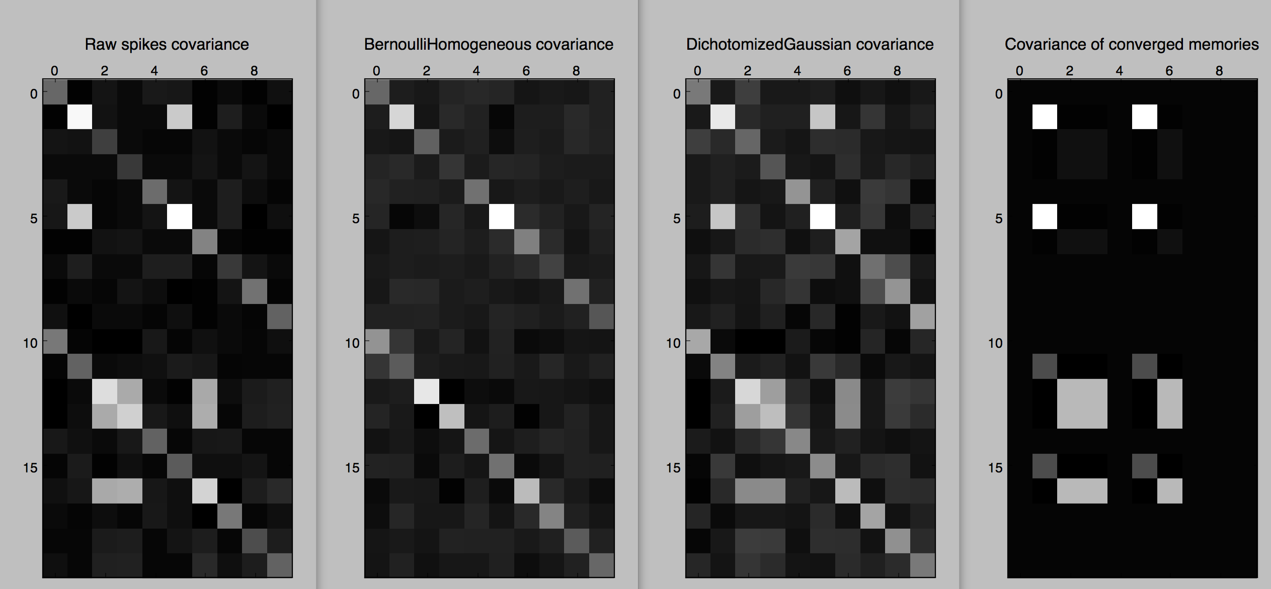
Figure 2. Covariances of two trials with 10 neurons.

As we can see in Figures 1 and 2, the samples from Bernoulli have the correct firing rates in each trial, but not the coordinated aspect (as can be seen in the covariance matrices for each trial, which are basically diagonal matrices). A better model that keeps track of the correlations is the Dichotomized Gaussian [Bethge2008]:

# let's model them as DichotomizedGaussian:
# from the paper: Generating spike-trains with specified correlations, Macke et al.
spikes_model = DichotomizedGaussian(spikes=spikes)
DG_sample_spikes = spikes_model.sample_from_model()

plt.figure()
plt.title('DichotomizedGaussian sample')
plt.matshow(DG_sample_spikes.rasterize(), cmap='gray')

plt.figure()
plt.matshow(DG_sample_spikes.covariance().reshape((2 * 10, 10)), cmap='gray')
plt.title('DichotomizedGaussian covariance')

plt.show()

Finally, we try and model the data with a Hopfield network trained using MPF [HS-DK201] over all the trials:

# the basic modeler trains a Hopfield network using MPF on the raw spikes
spikes_model = SpikeModel(spikes=spikes)
spikes_model.fit()  # note: this fits a single network to all trials
spikes_model.chomp()

converged_spikes = Spikes(spikes=spikes_model.hopfield_spikes)

plt.figure()
plt.title('Converge dynamics on Raw data')
plt.matshow(converged_spikes.rasterize(), cmap='gray')

plt.figure()
plt.title('Covariance of converged memories')
plt.matshow(converged_spikes.covariance().reshape((2 * 10, 10)), cmap='gray')

plt.show()

Going further

One thing we would like to do is examine the structure of the memories:

# plot memory label (its chronological appearance) as a function of time
plt.figure()
plt.scatter(range(len(spikes_model.memories.sequence)), 1 + np.array(spikes_model.memories.sequence))
plt.xlabel('time bin')
plt.ylabel('Memory number (chronological order of appearance)')
plt.title('Converged memory label at each time bin')

# versus the raw data
plt.figure()
plt.scatter(range(len(spikes_model.empirical.sequence)), 1 + np.array(spikes_model.empirical.sequence))
plt.ylabel('Raw pattern number (chronological order of appearance)')
plt.xlabel('time bin')
plt.title('Raw pattern label at each time bin')

plt.show()

Notice in Figures 4 and 4 that the converged dynamics of the trained Hopfield network on the original data does reveal the hidden assemblies for the most part.

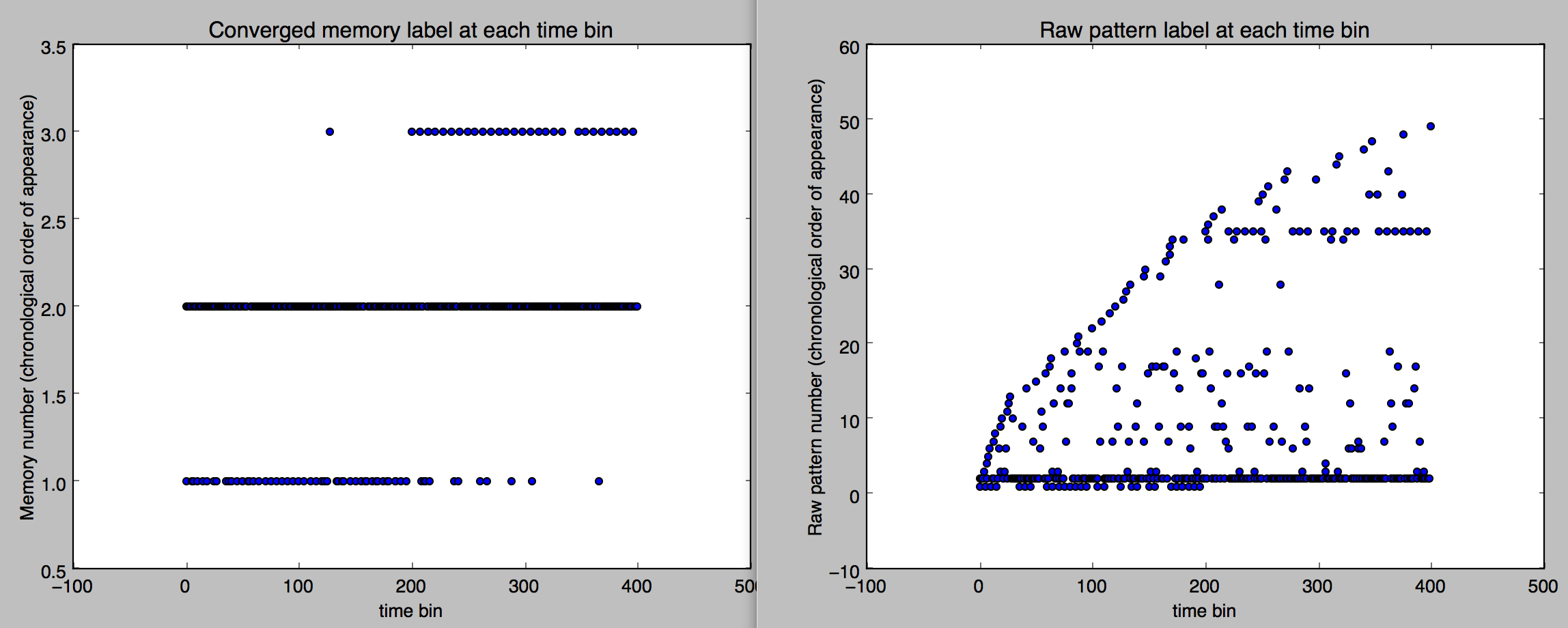
Figure 3. Patterns (converged at left, raw on right) over time bins labeled on the vertical axis by their first appearance in the dataset.

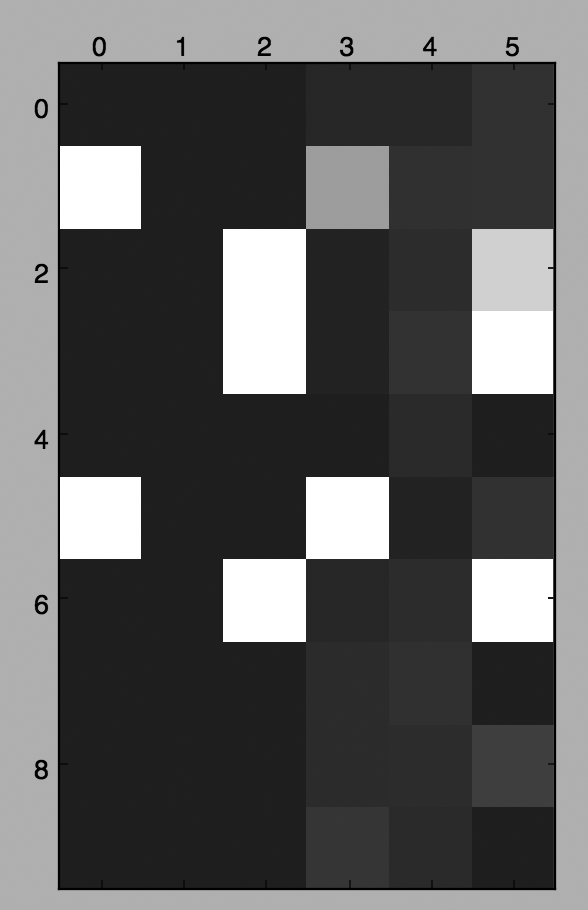
Figure 4. Memories in network (left) and Memory Triggered Averages (at right)

Now that we know there are basically two assemblies, one showing up lots in the first trial and the other in the second, let’s look at the memories and their corresponding Memory Triggered Averages MTAs that are obtained for each memory by averaging all raw patterns that converge to the given memory under the Hopfield dynamics.

The code below generates Fig. 2, which displaysa matrix whose first 3 columns are the memories in the network and whose next 3 columns are the average of raw data patterns converging to the corresponding memory in the first 3 columns:

# memories are ordered by their first appearance
bin_memories = spikes_model.memories.patterns
arr = np.zeros((spikes_model.original_spikes.N, 2 * len(bin_memories)))
for c, memory in enumerate(bin_memories):
    arr[:, c] = spikes_model.memories.fp_to_binary_matrix(c)

for c, memory in enumerate(bin_memories):
    arr[:, c + len(bin_memories)] = spikes_model.memories.mtas[memory] /
            spikes_model.memories.counts[memory]

print "Probabilities of each memory:"
print zip(bin_memories, spikes_model.memories.to_prob_vect())

# Probabilities of each memory:
# [('0100010000', 0.13), ('0000000000', 0.79249999999999998), /
# ('0011001000', 0.077499999999999999)]

Notice that the number of occurrences of the cell assembly with neuron 1 and 5 co-active is about double that of 2, 3, 6 co-active, consistent with our construction.

Saving and loading

One can save Spikes, Learner`s and :class:.SpikesModel`s:

spikes_model.save('my_spikes_model')
loaded_spikes_model = SpikesModel.load('my_spikes_model')

Note that a SpikesModel already keeps track of the original spikes it was constructed from and all other internal objects (such as the Hopfield network).

Stimuli

Continuing our example, we now discuss how to incorporate stimuli into our analyses.

First, let’s create a fake stimulus consisting of random normal 90 x 100 dimensional numpy arrays unless the fake stimulus is presented, in which case it is either a picture of Hobbes or Calvin (with some small noise added):

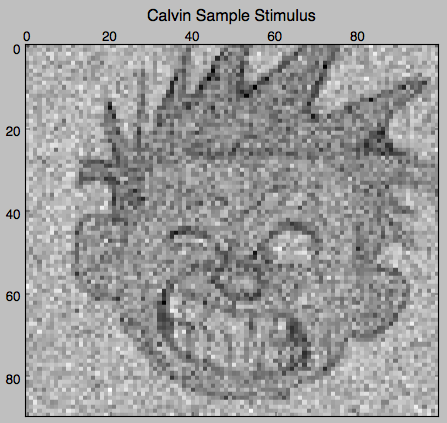
Figure 5. Noisy stimulus: Calvin.

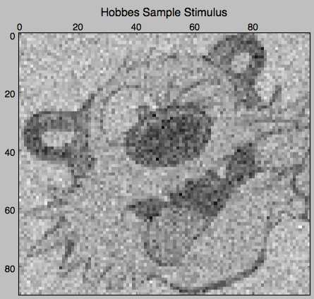
Figure 6. Noisy stimulus: Hobbes.

In code this looks like this:

from hdnet.stimulus import Stimulus

calvin = np.load('data/calvin.npy')  # 90 by 100 numpy array
hobbes = np.load('data/hobbes.npy')

stimulus_arr = 20 \* np.random.randn(2, 200, \*calvin.shape)
stimulus_arr[0, ::5] = calvin + 50 \* np.random.randn(200 / 5, \*calvin.shape)
stimulus_arr[1, ::11] = hobbes + 50 \* np.random.randn(200 / 11 + 1, /
                        \*hobbes.shape)

plt.matshow(stimulus_arr[0, 0], cmap='gray')
plt.title('Calvin Sample Stimulus')
plt.matshow(stimulus_arr[1, 0], cmap='gray')
plt.title('Hobbes Sample Stimulus')

Now, let’s try and see what were the average stimuli for each fixed-point / memory. We call such features Memory Triggered Stimulus Averages (MTSA):

stimulus = Stimulus(stimulus_arr=stimulus_arr)
avgs = spikes_model.memories.mem_triggered_stim_avgs(stimulus)

for stm_avg in avgs:
    plt.figure()
    plt.matshow(stm_avg, cmap='gray')
    plt.title('Memory Triggered Stimulus Average')

plt.show()

The MTSAs look as following.

Figure 7. Memory-triggered-stimulus averages of the Calvin spike pattern in the data.

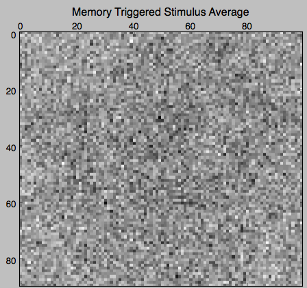
Figure 8. Memory-triggered-stimulus averages of the empty spike pattern in the data.

Figure 9. Memory-triggered-stimulus averages of the Hobbes spike pattern in the data.

Real data

Now, we try these methods out on some real data. First, we download polytrode data recorded by Tim Blanche in the laboratory of Nicholas Swindale, University of British Columbia from the NSF-funded CRCNS Data Sharing website

Let’s examine the spontaneous spiking data from anesthetized cat visual cortex area 18 (around 5 minutes of spike-sorted polytrode data from 50 neurons).

First we read the data using the .spk format reader integrated in hdnet:

from hdnet.data import SpkReader
fn = 'data/Blanche/crcns_pvc3_cat_recordings/drifting_bar/spike_data'
spikes = SpkReader.read_spk_folder(fn)

Now we fit a Hopfield network on the spike data:

spikes_model = SpikeModel(spikes=spikes)
spikes_model.fit()  # note: this fits a single network to all trials

After fitting the model we converge the windows of raw data to their Hopfield memories:

spikes_model.chomp()
converged_spikes = Spikes(spikes=spikes_model.hopfield_spikes)

We can now plot them and their covariance:

plt.matshow(converged_spikes.rasterize(), cmap='gray')
plt.title('Converge dynamics on Raw data')
plt.matshow(converged_spikes.covariance().reshape((2 * 10, 10)), cmap='gray')
plt.title('Covariance of converged memories')

TBC